Quantum Gates¶

In [1]:

import numpy as np
from qutip import tensor, basis, ket2dm, average_gate_fidelity, Qobj
from qutip_qip.circuit import QubitCircuit
from chalmers_qubit.devices.sarimner import *
from chalmers_qubit.utils.operations import project_on_qubit

import warnings
warnings.simplefilter(action="ignore", category=FutureWarning)

%load_ext autoreload
%autoreload 2

import numpy as np from qutip import tensor, basis, ket2dm, average_gate_fidelity, Qobj from qutip_qip.circuit import QubitCircuit from chalmers_qubit.devices.sarimner import * from chalmers_qubit.utils.operations import project_on_qubit import warnings warnings.simplefilter(action="ignore", category=FutureWarning) %load_ext autoreload %autoreload 2

Single Qubit Gate Example¶

We begin by creating a quantum circuit that has a single-qubit, and we perform a single-qubit gate on it

In [2]:

num_qubits = 1
circuit = QubitCircuit(num_qubits)
circuit.add_gate("RX", targets=0, arg_value=np.pi)

num_qubits = 1 circuit = QubitCircuit(num_qubits) circuit.add_gate("RX", targets=0, arg_value=np.pi)

Next we define the hardware parameters that we will use when simulating this quantum circtuit. We therefore define a dictionary where the key corresponds to the qubit index and the value is another dict that can have the following values:

• frequency: Qubit frequency in GHz.
• anharmonicity: Qubit anharmonicity in GHz.

We will also create another dict with the decoherence values for the qubit, the key needs to match the qubit index, and the value is another dict with the relaxation times

• t1: $T_1$ of the qubit in nano seconds.
• t2: $T_2$ of the qubit in nano seconds.

In [3]:

transmon_dict = {
    0: {"frequency": 5.0, "anharmonicity": -0.30},
}
decoherence_dict = {
    0: {"t1": 60e3, "t2": 100e3},
}

transmon_dict = { 0: {"frequency": 5.0, "anharmonicity": -0.30}, } decoherence_dict = { 0: {"t1": 60e3, "t2": 100e3}, }

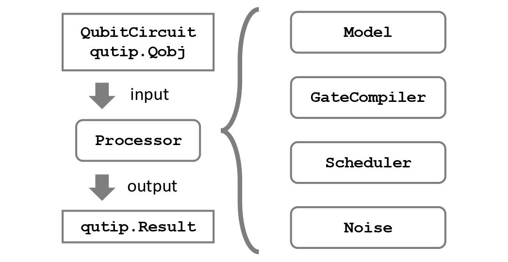
Next we take these hardware parameters that we have defined and we load them into our superconducting hardware model SarimnerModel. The SarimnerModel along with the SarimnerCompiler and noise are given to SarimnerProcessor as shown in the figure below.

In [4]:

# Load the physical parameters onto the model
model = SarimnerModel(transmon_dict=transmon_dict)

# Choose compiler
compiler = SarimnerCompiler(model=model)

# Add noise
noise = [DecoherenceNoise(decoherence_dict=decoherence_dict)]

# Create the processor with the given hardware parameters
sarimner = SarimnerProcessor(model=model, compiler=compiler, noise=noise)

# Load the physical parameters onto the model model = SarimnerModel(transmon_dict=transmon_dict) # Choose compiler compiler = SarimnerCompiler(model=model) # Add noise noise = [DecoherenceNoise(decoherence_dict=decoherence_dict)] # Create the processor with the given hardware parameters sarimner = SarimnerProcessor(model=model, compiler=compiler, noise=noise)

Once we have defined our processor we can load the quantum circuit onto the processor. This will compile the circuit into a pulse sequence.

In [5]:

tlist, coeffs = sarimner.load_circuit(circuit)

tlist, coeffs = sarimner.load_circuit(circuit)

We can choose to plot the pulse sequence

In [6]:

fig, ax = sarimner.plot_pulses(show_axis=True, figsize=(6,3));

fig, ax = sarimner.plot_pulses(show_axis=True, figsize=(6,3));

Now we can exectue this pulse sequence on the processor by using run_state with a given initial state

In [7]:

initial_state = basis(3,0)
result = sarimner.run_state(initial_state)
final_state = result.states[-1]
final_state

initial_state = basis(3,0) result = sarimner.run_state(initial_state) final_state = result.states[-1] final_state

Out[7]:

Quantum object: dims=[[3], [3]], shape=(3, 3), type='oper', dtype=Dense, isherm=True$$\left(\begin{array}{cc}3.966\times10^{ -4 } & 0.002j & 2.968\times10^{ -8 }\\-0.002j & 1.000 & 3.140\times10^{ -7 }\\2.968\times10^{ -8 } & 3.140\times10^{ -7 } & 1.327\times10^{ -7 }\end{array}\right)$$

Since we simulated the system for a three-level system we have to project it onto the computational subspace using the function project_on_qubit

In [8]:

project_on_qubit(final_state)

project_on_qubit(final_state)

Out[8]:

Quantum object: dims=[[2], [2]], shape=(2, 2), type='oper', dtype=Dense, isherm=True$$\left(\begin{array}{cc}3.966\times10^{ -4 } & 0.002j\\-0.002j & 1.000\end{array}\right)$$

Two Qubit Gate Example¶

Next we show a simple circuit using a two-qubit CZ-gate and how to compile it onto our processor.

In [9]:

# Define a circuit and run the simulation
num_qubits = 2
circuit = QubitCircuit(num_qubits)
circuit.add_gate("CZ", controls=0, targets=1)

# Define a circuit and run the simulation num_qubits = 2 circuit = QubitCircuit(num_qubits) circuit.add_gate("CZ", controls=0, targets=1)

Just as before we start by defining our hardware parameters.

In [10]:

transmon_dict = {
    0: {"frequency": 5.0, "anharmonicity": -0.30},
    1: {"frequency": 5.4, "anharmonicity": -0.30},
}
decoherence_dict = {
    0: {"t1": 60e3, "t2": 80e3},
    1: {"t1": 100e3, "t2": 105e3},
}

transmon_dict = { 0: {"frequency": 5.0, "anharmonicity": -0.30}, 1: {"frequency": 5.4, "anharmonicity": -0.30}, } decoherence_dict = { 0: {"t1": 60e3, "t2": 80e3}, 1: {"t1": 100e3, "t2": 105e3}, }

Additionally we need to supply information of how the qubits are coupled together. This is done using another dictionary, where the value is supplied as a tuple (i,j) defining qubit $i$ and qubit $j$ and the value is the coupling strength in GHz.

In [11]:

# The time for the CZ-gate that we want in (ns)
t = 100

# Corresponding coupling in (GHz)
g = 1 / (np.sqrt(2) * 2 * t)

coupling_dict = {
    (0, 1): g,
}

# The time for the CZ-gate that we want in (ns) t = 100 # Corresponding coupling in (GHz) g = 1 / (np.sqrt(2) * 2 * t) coupling_dict = { (0, 1): g, }

and load them onto our model

In [12]:

# Load the physical parameters onto the model
model = SarimnerModel(transmon_dict=transmon_dict, coupling_dict=coupling_dict)
# Options for compiler
options = {
    "dt": 0.1, # time-step of simulator in (ns)
    "two_qubit_gate": {
        "buffer_time": 10, # buffer-time of two-qubit gate in (ns)
        "rise_fall_time": 0, # sinusodial rise and fall time of two-qubit gate in (ns)
    },
}
# Choose compiler
compiler = SarimnerCompiler(model=model, options=options)
# Create the processor with the given hardware parameters
sarimner = SarimnerProcessor(model=model, compiler=compiler)

# Load the physical parameters onto the model model = SarimnerModel(transmon_dict=transmon_dict, coupling_dict=coupling_dict) # Options for compiler options = { "dt": 0.1, # time-step of simulator in (ns) "two_qubit_gate": { "buffer_time": 10, # buffer-time of two-qubit gate in (ns) "rise_fall_time": 0, # sinusodial rise and fall time of two-qubit gate in (ns) }, } # Choose compiler compiler = SarimnerCompiler(model=model, options=options) # Create the processor with the given hardware parameters sarimner = SarimnerProcessor(model=model, compiler=compiler)

Then we can compile the circuit onto our processor

In [13]:

tlist, coeffs = sarimner.load_circuit(circuit)

tlist, coeffs = sarimner.load_circuit(circuit)

In [14]:

cz_real, cz_imag = coeffs["cz_real01"], coeffs["cz_imag01"]
cz = np.sqrt(cz_real**2 + cz_imag**2)
tlist_real, tlist_imag = tlist["cz_real01"], tlist["cz_imag01"]

cz_real, cz_imag = coeffs["cz_real01"], coeffs["cz_imag01"] cz = np.sqrt(cz_real**2 + cz_imag**2) tlist_real, tlist_imag = tlist["cz_real01"], tlist["cz_imag01"]

In [15]:

np.trapezoid(cz, tlist_real)

np.trapezoid(cz, tlist_real)

Out[15]:

np.float64(100.0)

In [16]:

area = np.trapezoid(y=cz_real, x=tlist_real) + np.trapezoid(y=cz_real, x=tlist_real)

area = np.trapezoid(y=cz_real, x=tlist_real) + np.trapezoid(y=cz_real, x=tlist_real)

In [17]:

sarimner.plot_pulses(show_axis=True, figsize=(6,3));

sarimner.plot_pulses(show_axis=True, figsize=(6,3));

To see that the CZ-gate is implemented correctly we will now simulate the circuit using the master equation simulation and look at the expectation values of the $|11\rangle$ and $|20\rangle$ states.

In [18]:

ket01 = tensor(basis(3,0), basis(3,1))
ket10 = tensor(basis(3,1), basis(3,0))
ket11 = tensor(basis(3,1), basis(3,1))
ket20 = tensor(basis(3,2), basis(3,0))
# List of operators we wanna compute the expectation value for during the simulation
e_ops = [ket2dm(ket01), ket2dm(ket10), ket2dm(ket11), ket2dm(ket20)]
result = sarimner.run_state(ket11, e_ops=e_ops, options={'nsteps': 1e5, 'store_final_state': True})

ket01 = tensor(basis(3,0), basis(3,1)) ket10 = tensor(basis(3,1), basis(3,0)) ket11 = tensor(basis(3,1), basis(3,1)) ket20 = tensor(basis(3,2), basis(3,0)) # List of operators we wanna compute the expectation value for during the simulation e_ops = [ket2dm(ket01), ket2dm(ket10), ket2dm(ket11), ket2dm(ket20)] result = sarimner.run_state(ket11, e_ops=e_ops, options={'nsteps': 1e5, 'store_final_state': True})

In [19]:

import matplotlib.pyplot as plt
plt.plot(result.times, result.expect[0], label="01")
plt.plot(result.times, result.expect[1], label="10")
plt.plot(result.times, result.expect[2], label='11')
plt.plot(result.times, result.expect[3], label='20')
plt.xlabel('Time (ns)')
plt.ylabel('Population')
plt.legend()

import matplotlib.pyplot as plt plt.plot(result.times, result.expect[0], label="01") plt.plot(result.times, result.expect[1], label="10") plt.plot(result.times, result.expect[2], label='11') plt.plot(result.times, result.expect[3], label='20') plt.xlabel('Time (ns)') plt.ylabel('Population') plt.legend()

Out[19]:

<matplotlib.legend.Legend at 0x163760400>

And if we print the final state we see that the $|11\rangle$ state has the desired $-1$ phase.

In [20]:

qubit_state = project_on_qubit(result.final_state)
qubit_state

qubit_state = project_on_qubit(result.final_state) qubit_state

Out[20]:

Quantum object: dims=[[2, 2], [1, 1]], shape=(4, 1), type='ket', dtype=Dense$$\left(\begin{array}{cc}0\\0\\0\\-1.000\end{array}\right)$$

Three Qubit Gate Example¶

Finally we will demonstrate the implementation of the three-qubit gate.

Since this gate is not part of qutip QubitCircuit we have to defined the gate ourself and supply as user_gates

In [21]:

from qutip import Qobj
# Ideal gate
def cczs(args):
    theta, phi, gamma = args
    U = np.array([[1, 0, 0, 0, 0, 0, 0, 0],
                  [0, 1, 0, 0, 0, 0, 0, 0],
                  [0, 0, 1, 0, 0, 0, 0, 0],
                  [0, 0, 0, 1, 0, 0, 0, 0],
                  [0, 0, 0, 0, 1, 0, 0, 0],
                  [0, 0, 0, 0, 0, -np.exp(-1j*gamma)*np.sin(theta/2)**2 + np.cos(theta/2)**2, 
                                    (1/2)*(1 + np.exp(-1j*gamma))*np.exp(-1j*phi)*np.sin(theta), 0],
                  [0, 0, 0, 0, 0, (1/2)*(1 + np.exp(-1j*gamma))*np.exp(1j*phi)*np.sin(theta), 
                                    -np.exp(-1j*gamma)*np.cos(theta/2)**2 + np.sin(theta/2)**2, 0],
                  [0, 0, 0, 0, 0, 0, 0, -np.exp(1j*gamma)]], dtype="complex")
    return Qobj(U, dims=[[2]*3, [2]*3])

from qutip import Qobj # Ideal gate def cczs(args): theta, phi, gamma = args U = np.array([[1, 0, 0, 0, 0, 0, 0, 0], [0, 1, 0, 0, 0, 0, 0, 0], [0, 0, 1, 0, 0, 0, 0, 0], [0, 0, 0, 1, 0, 0, 0, 0], [0, 0, 0, 0, 1, 0, 0, 0], [0, 0, 0, 0, 0, -np.exp(-1j*gamma)*np.sin(theta/2)**2 + np.cos(theta/2)**2, (1/2)*(1 + np.exp(-1j*gamma))*np.exp(-1j*phi)*np.sin(theta), 0], [0, 0, 0, 0, 0, (1/2)*(1 + np.exp(-1j*gamma))*np.exp(1j*phi)*np.sin(theta), -np.exp(-1j*gamma)*np.cos(theta/2)**2 + np.sin(theta/2)**2, 0], [0, 0, 0, 0, 0, 0, 0, -np.exp(1j*gamma)]], dtype="complex") return Qobj(U, dims=[[2]*3, [2]*3])

Alternatively we can just import the gate from chalmers_qubit.utils.gates

In [22]:

from chalmers_qubit.utils.gates import cczs

from chalmers_qubit.utils.gates import cczs

In [23]:

# Define a circuit and run the simulation
num_qubits = 3

circuit = QubitCircuit(num_qubits)
circuit.user_gates = {"CCZS": cczs}
circuit.add_gate("CCZS", targets=[0,1,2], arg_value=[np.pi/2,0,0])

# Define a circuit and run the simulation num_qubits = 3 circuit = QubitCircuit(num_qubits) circuit.user_gates = {"CCZS": cczs} circuit.add_gate("CCZS", targets=[0,1,2], arg_value=[np.pi/2,0,0])

In [24]:

transmon_dict = {
            0: {"frequency": 5.0, "anharmonicity": 0.3},
            1: {"frequency": 5.4, "anharmonicity": 0.3},
            2: {"frequency": 5.2, "anharmonicity": 0.3},
        }

# Times in (ns)
t = 100

# corresponding coupling
g = 1 / (np.sqrt(2) * 2 * t)

coupling_dict = {(0, 1): g,
                 (0, 2): -g} # for phi=0 the coupling strengths need different signs

transmon_dict = { 0: {"frequency": 5.0, "anharmonicity": 0.3}, 1: {"frequency": 5.4, "anharmonicity": 0.3}, 2: {"frequency": 5.2, "anharmonicity": 0.3}, } # Times in (ns) t = 100 # corresponding coupling g = 1 / (np.sqrt(2) * 2 * t) coupling_dict = {(0, 1): g, (0, 2): -g} # for phi=0 the coupling strengths need different signs

In [25]:

# Load the physical parameters onto the model
model = SarimnerModel(
    transmon_dict=transmon_dict,
    coupling_dict=coupling_dict
)
options = {
    "dt": 0.1,
    "two_qubit_gate": {
        "buffer_time": 0,
        "rise_fall_time": 0.1,
    },
}
# Choose compiler
compiler = SarimnerCompiler(model=model, options=options)
# Create the processor with the given hardware parameters
sarimner = SarimnerProcessor(model=model, compiler=compiler, noise=[])

# Load the physical parameters onto the model model = SarimnerModel( transmon_dict=transmon_dict, coupling_dict=coupling_dict ) options = { "dt": 0.1, "two_qubit_gate": { "buffer_time": 0, "rise_fall_time": 0.1, }, } # Choose compiler compiler = SarimnerCompiler(model=model, options=options) # Create the processor with the given hardware parameters sarimner = SarimnerProcessor(model=model, compiler=compiler, noise=[])

In [26]:

tlist, coeffs = sarimner.load_circuit(circuit)

tlist, coeffs = sarimner.load_circuit(circuit)

In [27]:

sarimner.plot_pulses(show_axis=True);

sarimner.plot_pulses(show_axis=True);

In [28]:

ket110 = tensor([basis(3,1),basis(3,1),basis(3,0)])
ket101 = tensor([basis(3,1),basis(3,0),basis(3,1)])
ket200 = tensor([basis(3,2),basis(3,0),basis(3,0)])
e_ops = [ket2dm(ket110), ket2dm(ket101), ket2dm(ket200)]
result = sarimner.run_state(ket110, e_ops=e_ops, options={'store_states':True, 'nsteps':1e5, 'atol': 1e-12})

ket110 = tensor([basis(3,1),basis(3,1),basis(3,0)]) ket101 = tensor([basis(3,1),basis(3,0),basis(3,1)]) ket200 = tensor([basis(3,2),basis(3,0),basis(3,0)]) e_ops = [ket2dm(ket110), ket2dm(ket101), ket2dm(ket200)] result = sarimner.run_state(ket110, e_ops=e_ops, options={'store_states':True, 'nsteps':1e5, 'atol': 1e-12})

In [29]:

import matplotlib.pyplot as plt
plt.plot(result.times,result.expect[0], label="110")
plt.plot(result.times,result.expect[1], label="101")
plt.plot(result.times,result.expect[2], label="200")
plt.legend()

import matplotlib.pyplot as plt plt.plot(result.times,result.expect[0], label="110") plt.plot(result.times,result.expect[1], label="101") plt.plot(result.times,result.expect[2], label="200") plt.legend()

Out[29]:

<matplotlib.legend.Legend at 0x1640576d0>

Using the run_propagator method we can compute the propagator of the evolution.

In [30]:

prop = sarimner.run_propagator(options={"nsteps":1e5})
prop = project_on_qubit(prop)
prop

prop = sarimner.run_propagator(options={"nsteps":1e5}) prop = project_on_qubit(prop) prop

Out[30]:

Quantum object: dims=[[2, 2, 2], [2, 2, 2]], shape=(8, 8), type='oper', dtype=Dense, isherm=False$$\left(\begin{array}{cc}1 & 0 & 0 & 0 & 0 & 0 & 0 & 0\\0 & 1 & 0 & 0 & 0 & 0 & 0 & 0\\0 & 0 & 1 & 0 & 0 & 0 & 0 & 0\\0 & 0 & 0 & 1 & 0 & 0 & 0 & 0\\0 & 0 & 0 & 0 & 1 & 0 & 0 & 0\\0 & 0 & 0 & 0 & 0 & 6.671\times10^{ -6 } & 1.000 & 0\\0 & 0 & 0 & 0 & 0 & 1.000 & 6.671\times10^{ -6 } & 0\\0 & 0 & 0 & 0 & 0 & 0 & 0 & -1.000\end{array}\right)$$

We can then compute the average gate fidelity between the ideal gate and the simulated gate

In [31]:

ideal_prop = cczs((np.pi / 2, 0, 0))
average_gate_fidelity(ideal_prop, prop)

ideal_prop = cczs((np.pi / 2, 0, 0)) average_gate_fidelity(ideal_prop, prop)

Out[31]:

np.float64(0.9999940699864269)